Assignment 1: Solutions
Read the data
library("readr")
df = read_csv("https://raw.githubusercontent.com/MuseumofModernArt/collection/master/Artworks.csv")
Question 1: Create a new dataframe of the stock of paintings at MOMA for each month in the year
library("dplyr")
library("lubridate")
library("zoo")

df.q1 = df %>%
  mutate(
    year = year(DateAcquired),
    month = month(DateAcquired),
    date = ymd(paste(year, month, "01",sep = "-"))
  ) %>%
  group_by(date) %>%
  summarise(
    supply = n()
  ) %>%
  arrange(date) %>%
  mutate(
    stock = cumsum(supply)
  )
head(df.q1)
## Source: local data frame [6 x 3]
##
## date supply stock
## (time) (int) (int)
## 1 1929-11-01 9 9
## 2 1930-01-01 3 12
## 3 1930-04-01 2 14
## 4 1930-06-01 1 15
## 5 1930-10-01 2 17
## 6 1931-01-01 2 19Question 2: Use ggplot2 and your new data frame to plot the the stock of paintings on the y-axis and the date on the x-axis
library("zoo")
library("ggplot2")
library("ggthemes")
library("scales")
library("viridis")

p = ggplot(df.q1, aes(x = date, y = stock))
p + geom_line(colour = "red", size = 1) +
  theme_tufte() +
  theme(axis.title = element_text(),
        axis.title.y = element_text(angle = 90)) +
  labs("stock of paintings", title = "Question 2", x = NULL) +
scale_y_continuous(labels=comma) 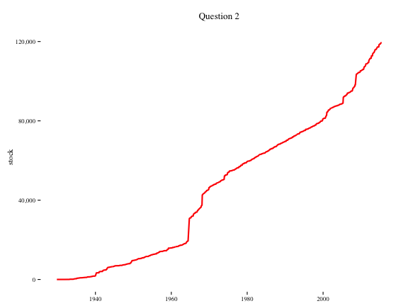
Question 3: Create the same plot but this time the color should reflect the stock of paintings for curator approved and non-curator approved paintings, respectively
df.q3 = df %>%
  mutate(
    year = year(DateAcquired),
    month = month(DateAcquired),
    date = ymd(paste(year, month, "01",sep = "-"))
  ) %>%
  group_by(date, CuratorApproved) %>%
  summarise(
    supply = n()
  ) %>%
  ungroup() %>%
  group_by(CuratorApproved) %>%
  arrange(CuratorApproved, date) %>%
  mutate(
    stock = cumsum(supply)
  )
head(df.q3)
## Source: local data frame [6 x 4]
## Groups: CuratorApproved [1]
##
## date CuratorApproved supply stock
## (time) (chr) (int) (int)
## 1 1931-01-01 N 1 1
## 2 1932-12-01 N 1 2
## 3 1933-01-01 N 1 3
## 4 1933-04-01 N 90 93
## 5 1934-04-01 N 14 107
## 6 1934-05-01 N 65 172p = ggplot(df.q3, aes(x = date, y = stock, colour = CuratorApproved))
p + geom_line(size = 1) +
theme_tufte() +
theme(axis.title = element_text(),
axis.title.y = element_text(angle = 90)) +
labs("stock of paintings", title = "Question 3", x = NULL) +
scale_y_continuous(labels=comma) +
scale_color_viridis(discrete = TRUE)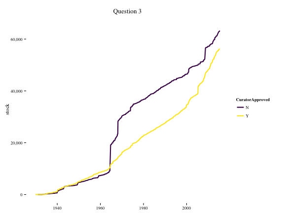
Question 4: Create a new data frame of the stock of paintings grouped by what department the painting belongs to
df.q4 = df %>%
  mutate(
    year = year(DateAcquired),
    month = month(DateAcquired),
    date = ymd(paste(year, month, "01",sep = "-"))
  ) %>%
  group_by(date, Department) %>%
  summarise(
    supply = n()
  ) %>%
  ungroup() %>%
  group_by(Department) %>%
  arrange(Department, date) %>%
  mutate(
    stock = cumsum(supply)
  )
head(df.q4)
## Source: local data frame [6 x 4]
## Groups: Department [1]
##
## date Department supply stock
## (time) (chr) (int) (int)
## 1 1932-01-01 Architecture & Design 2 2
## 2 1934-01-01 Architecture & Design 2 4
## 3 1934-04-01 Architecture & Design 43 47
## 4 1934-09-01 Architecture & Design 4 51
## 5 1935-11-01 Architecture & Design 22 73
## 6 1935-12-01 Architecture & Design 1 74Question 5: Plot this data frame using ggplot2. Which department has had the highest increase in their stock of paintings?
p = ggplot(df.q4, aes(x = date, y = stock, colour = Department))
p + geom_line(size = 1) +
  theme_tufte() +
  theme(axis.title = element_text(),
        axis.title.y = element_text(angle = 90)) +
  labs("stock of paintings", title = "Question 5", x = NULL) +
  scale_y_continuous(labels=comma) +
  scale_color_viridis(discrete = TRUE)
p = ggplot(df.q4, aes(x = date, y = stock, colour = Department))
p + geom_line(size = 1) +
  theme_tufte() +
  theme(axis.title = element_text(),
        axis.title.y = element_text(angle = 90)) +
  labs("stock of paintings", title = "Question 5", x = NULL) +
  scale_y_log10() +
  scale_color_viridis(discrete = TRUE)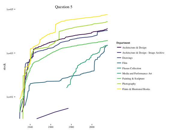
# Alternative:
df.q4.alt = df %>%
  group_by(Department) %>%
  summarise(
    stock = n()
  )
head(df.q4.alt)
## Source: local data frame [6 x 2]
##
## Department stock
## (chr) (int)
## 1 Architecture & Design 15828
## 2 Architecture & Design - Image Archive 18
## 3 Drawings 10738
## 4 Film 2587
## 5 Fluxus Collection 2547
## 6 Media and Performance Art 2350p = ggplot(df.q4.alt, aes(x = Department, y = stock, fill = Department))
p + geom_bar(stat="identity") +
theme_tufte() +
scale_y_continuous(labels=comma) +
theme(axis.text.x = element_blank(),
legend.position = "none") +
facet_wrap(~ Department, scales = "free_x") +
scale_fill_viridis(discrete = TRUE)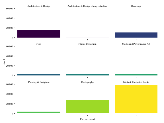
Question 6: Write a piece of code that counts the number of paintings by each artist in the data set. List the 10 painters with the highest number of paintings in MOMA’s collection.
df.artist = df %>%
  filter(Artist != "") %>%
  group_by(Artist) %>%
  summarise(count = n()) %>%
  arrange(-count)

head(df.artist, 10)
## Source: local data frame [10 x 2]
##
## Artist count
## (chr) (int)
## 1 Eugène Atget 5050
## 2 Louise Bourgeois 3224
## 3 Ludwig Mies van der Rohe 2497
## 4 Unknown photographer 1573
## 5 Jean Dubuffet 1426
## 6 Lee Friedlander 1317
## 7 Pablo Picasso 1309
## 8 Marc Chagall 1146
## 9 Henri Matisse 1064
## 10 Pierre Bonnard 940Question 7: The variable ArtistBio lists the birth place of each painter. Use this information to create a world map where each country is colored according to the stock of paintings in MOMA’s collection.
library("stringr")
df$Nationality = str_extract(df$ArtistBio, "[A-Z][a-z]+")

df.nationality = df %>%
  group_by(Nationality) %>%
  summarise(count = n())

head(df.nationality)
## Source: local data frame [6 x 2]
##
## Nationality count
## (chr) (int)
## 1 Active 3
## 2 Afghan 1
## 3 Albanian 23
## 4 Algerian 5
## 5 American 54031
## 6 Anglo 4Information on country and country adjective available here
Scrape and create data frame
library("rvest")
link = "https://www.englishclub.com/vocabulary/world-countries-nationality.htm"
css.selector = "td:nth-child(2) , td:nth-child(1)"

country = link %>%
  read_html() %>%
  html_nodes(css = "td:nth-child(1)") %>%
  html_text()

adjective = link %>%
  read_html() %>%
  html_nodes(css = "td:nth-child(2)") %>%
  html_text()

df.info = data.frame(country = country, adjective = adjective)
df.info$adjective = tolower(df.info$adjective)

df.info$adjective = ifelse(df.info$country == "United States of America (USA)",
                           "american", df.info$adjective)

head(df.info)
## country adjective
## 1 Afghanistan afghan
## 2 Albania albanian
## 3 Algeria algerian
## 4 Andorra andorran
## 5 Angola angolan
## 6 Argentina argentiniandf.nationality$Nationality = tolower(df.nationality$Nationality)
df.map = inner_join(df.nationality, df.info, by = c("Nationality" = "adjective"))
library("ggmap")
world.map = map_data("world")
library("countrycode")
world.map$iso2c = countrycode(world.map$region,
origin = "country.name",
destination = "iso2c")
df.map$iso2c = countrycode(df.map$country,
origin = "country.name",
destination = "iso2c")
df.map = inner_join(world.map, df.map, by = "iso2c")
p = ggplot(df.map, aes(x = long, y = lat, group = group, fill = count))
p + geom_polygon() +
theme_tufte() +
labs(title = "Painters by country") +
scale_fill_viridis()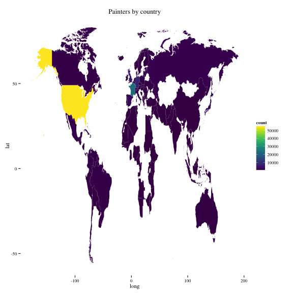
p = ggplot(df.map, aes(x = long, y = lat, group = group, fill = count))
p + geom_polygon() +
  theme_tufte() +
  labs(title = "Painters by country") +
  scale_fill_viridis(trans = "log", breaks = c(20, 8000),
                     labels = c("low", "high"),
                     name = "count\n(log transformed)")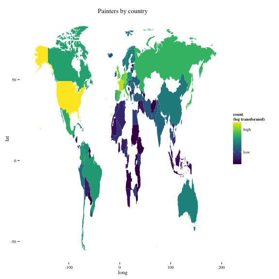
Question 8: The Dimensions variable lists the dimensions of each painting. Use your data manipulation skills to calculate the area of each painting (in cm’s). Create a data frame of the five largest and five smallest paintings in MOMA’s collection.
dim = str_extract(df$Dimensions, "\\([^()]+\\)")
dim = gsub("\\(|\\)", "", dim)
dim = gsub("[a-z]", "", dim)
dim = str_trim(dim)
dim = str_split(dim, "  ")
df$width = unlist(lapply(dim, function(x) x[1]))
df$length = unlist(lapply(dim, function(x) x[2]))
df$dim.length = unlist(lapply(dim, length))
df$height = NA
df$height[df$dim.length == 3] = unlist(lapply(dim[df$dim.length == 3],
                                              function(x) x[3]))
df = df %>%
  mutate(
    width = as.numeric(width),
    length = as.numeric(length),
    height = as.numeric(height),
    area = ifelse(dim.length == 3, width*length*height, width*length)
    )

summary(df$area)
## Min. 1st Qu. Median Mean 3rd Qu. Max. NA's
## 0.000e+00 3.530e+02 7.300e+02 9.604e+04 2.134e+03 1.419e+09 35288