Topic 1: Reading And Working With Data
In real life you will usually bring data into R from an outside file. This is rarely a pleasant experience, and we will devote several classes in a few weeks focused on how to clean and transform “messy” data. Since this is not our focus today, however, we will imagine all the data we work with today are “clean” (we will discuss what exactly “clean” and “messy” data is in the topic on data transformation).
What I want you to do before we meet is the following:
- Open up RStudio and type along while reading the text below. Try to think about what we’re doing instead of just zoning out and copying my code.
- Once you’ve done that, I want you to watch Reading/Writing Data: Part 1 and 2 by Roger Peng available here.
Usually, the data that you will work with can come from one of three sources1
- statistics packages (data generated from Stata, SAS, SPSS, etc)
- Excel
- flat files such as text files (
.txt) or comma separated value files (.csv)
Luckily, R has excellent capabilities for importing data from all sources listed above. I’ve created the following table to summarise the relevant options currently available in R
| Data | File Extension | Packages | Example |
|---|---|---|---|
| Statistical Packages | .dta (Stata) |
haven |
read_dta("path/to/file") |
.dta (Stata) |
foreign |
read.dta("path/to/file") |
|
.sas7bdat (SAS) |
haven |
read_sas("path/to/file") |
|
.sas7bdat (SAS) |
sas7bdat |
read.sas7bdat("path/to/file") |
|
| Excel | .xlsx |
readxl |
read_excel("path/to/file") |
.xlsx |
xlsx |
read.xlsx("path/to/file") |
|
| Flat files | .csv |
base |
read.csv("path/to/file") |
readr |
read_csv("path/to/file") |
||
.txt |
base |
read.table("path/to/file") |
The most common file format we will work with in this course is .csv.
Let us try to read a .csv file into R. For normal sized data you will most likely store this in a folder on your computer. For this example, however, I will read a dataset of battles in the Game of Thrones series available online here.
I use the readr library to read the data. To access this library we run the library("readr") function. The library must first be installed, however, which can be done by running the command install.packages("readr") or by accessing the Tools menu in RStudio, selecting Install Packages and typing in the name of the library.
library("readr")Afterwards, we can read the data
got.df = read_csv("https://raw.githubusercontent.com/chrisalbon/war_of_the_five_kings_dataset/master/5kings_battles_v1.csv")The read_csv function returns a data frame. There are many useful functions for getting a quick overview of the data. Here are just a few
names: lists the column names of the data framehead: lists the first five observationssummary: calcultes summary statistics for the variables in the data framedim: prints the number of rows and columns in the data frame
Any R code following a hash (#) is not executed. These are called comments, and can and should be used to annotate and explain your code. For example, this doesn’t do anything.
# this is a comment. R will not execute what I write hereLet us start by examining the dimensions of the data
dim(got.df)## [1] 38 25By running the command we learned that the data frame contains 38 rows and 25 columns.
Next, we print the column names
names(got.df)## [1] "name" "year" "battle_number"
## [4] "attacker_king" "defender_king" "attacker_1"
## [7] "attacker_2" "attacker_3" "attacker_4"
## [10] "defender_1" "defender_2" "defender_3"
## [13] "defender_4" "attacker_outcome" "battle_type"
## [16] "major_death" "major_capture" "attacker_size"
## [19] "defender_size" "attacker_commander" "defender_commander"
## [22] "summer" "location" "region"
## [25] "note"You can extract single variables and perform different operations on them. To extract a variable, we use the dollar sign ($). We can do more specific operations on this variable alone.
The Game of Thrones data holds detailed information on every major battle. Let us create some summary statistics for the size of the attacker’s force
summary(got.df$attacker_size)## Min. 1st Qu. Median Mean 3rd Qu. Max. NA's
## 20 1375 4000 9943 8250 100000 14We note that there are 14 missing observations (NAs) and that the mean size of the attackers force is 9,943.
The following build-in functions are useful for quickly summarizing a dataset
meanmedianminmaxquantile
When we have non-numeric variables, the table function is useful for quick counts
table(got.df$attacker_king)##
## Balon/Euron Greyjoy Joffrey/Tommen Baratheon
## 2 7 14
## Robb Stark Stannis Baratheon
## 10 5We see that “Joffrey/Tommen Baratheon” is the most aggressive character in the dataset, accounting for 14 of the 38 attacks in the data.
We can also get an idea of how succesfull each character is in their attacks by constructing a contingency table
table(got.df$attacker_king, got.df$attacker_outcome)##
## loss win
## 0 0 2
## Balon/Euron Greyjoy 0 0 7
## Joffrey/Tommen Baratheon 0 1 13
## Robb Stark 0 2 8
## Stannis Baratheon 1 2 2We see that Stannis Baratheon was the least succesful character in the data as he lost as many battles as he won.
Usually, it is much more productive to explore a dataset using visualisations instead of text and tables. In the next posts we will learn how to effectively visualise all kinds of data, but just to give you an idea of what is possible, I produce a few interesting plots of the data below.
We will use the plotting package ggplot2 for all the plotting in this course, so make sure this is installed if you want to run the code below
library("ggplot2")
p = ggplot(got.df, aes(x  = attacker_size,
  fill = attacker_king))
p = p + geom_density(alpha = .6) # add density geom
p = p + scale_x_log10() # transform x axis to log scale
p = p + labs(x = "size of attacking army (log scale)",
  title = "Whick king attacks with the largest army?")
plot(p)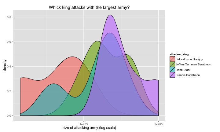
p = ggplot(subset(got.df, attacker_king != ""),
  aes( x = attacker_king))
p = p + geom_histogram() # add density geom
p = p + labs(x = "king",
  title = "Which king was most active in the war?")
plot(p)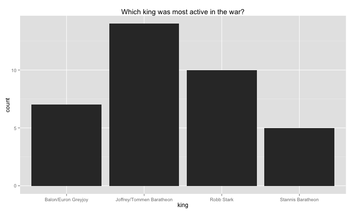
References
The Game of Thrones data used in this post is constructed by Chris Albion.
-
data can also come from databases such as SQL, but this is too advanced for our course. ↩